Latent Generative Anamorphoses
Code2D latent generative anamorphoses with Stable Diffusion 3.5, inspired by LookingGlass (CVPR2025)
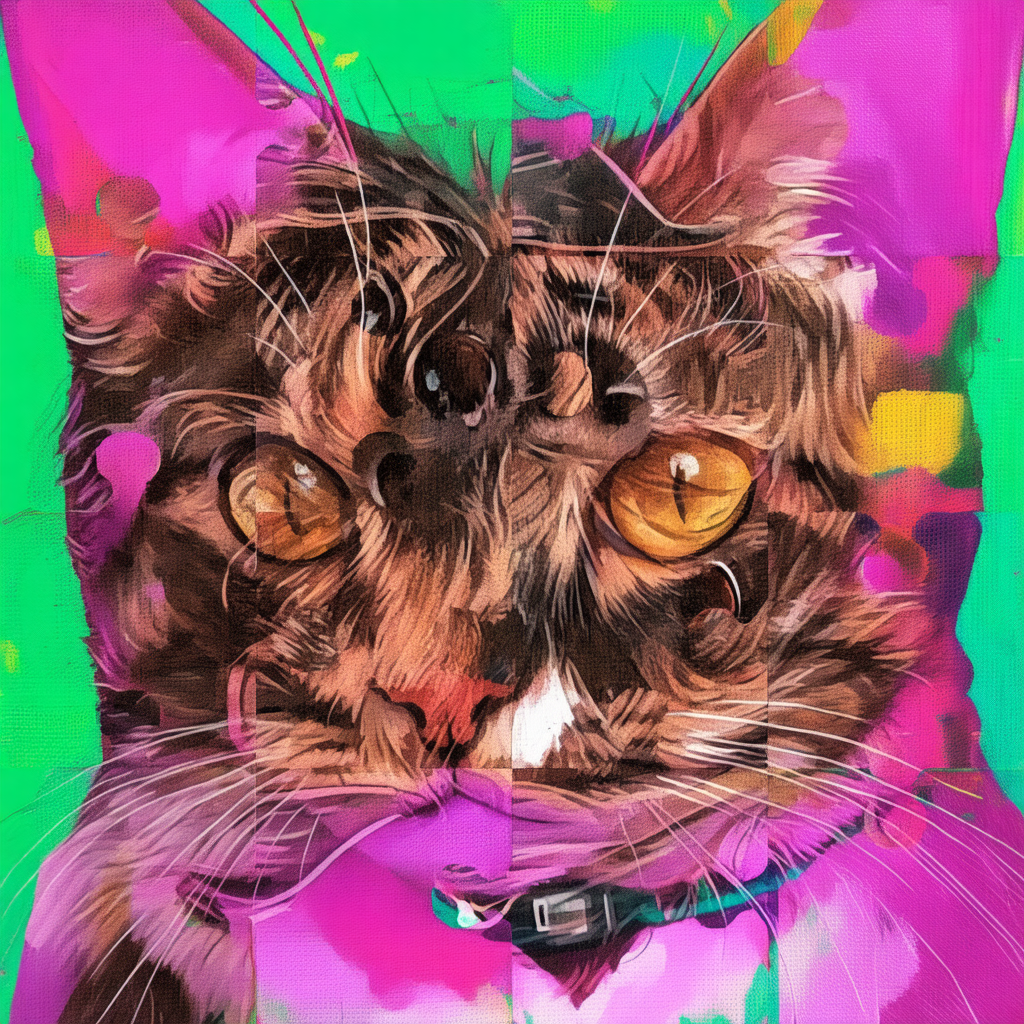
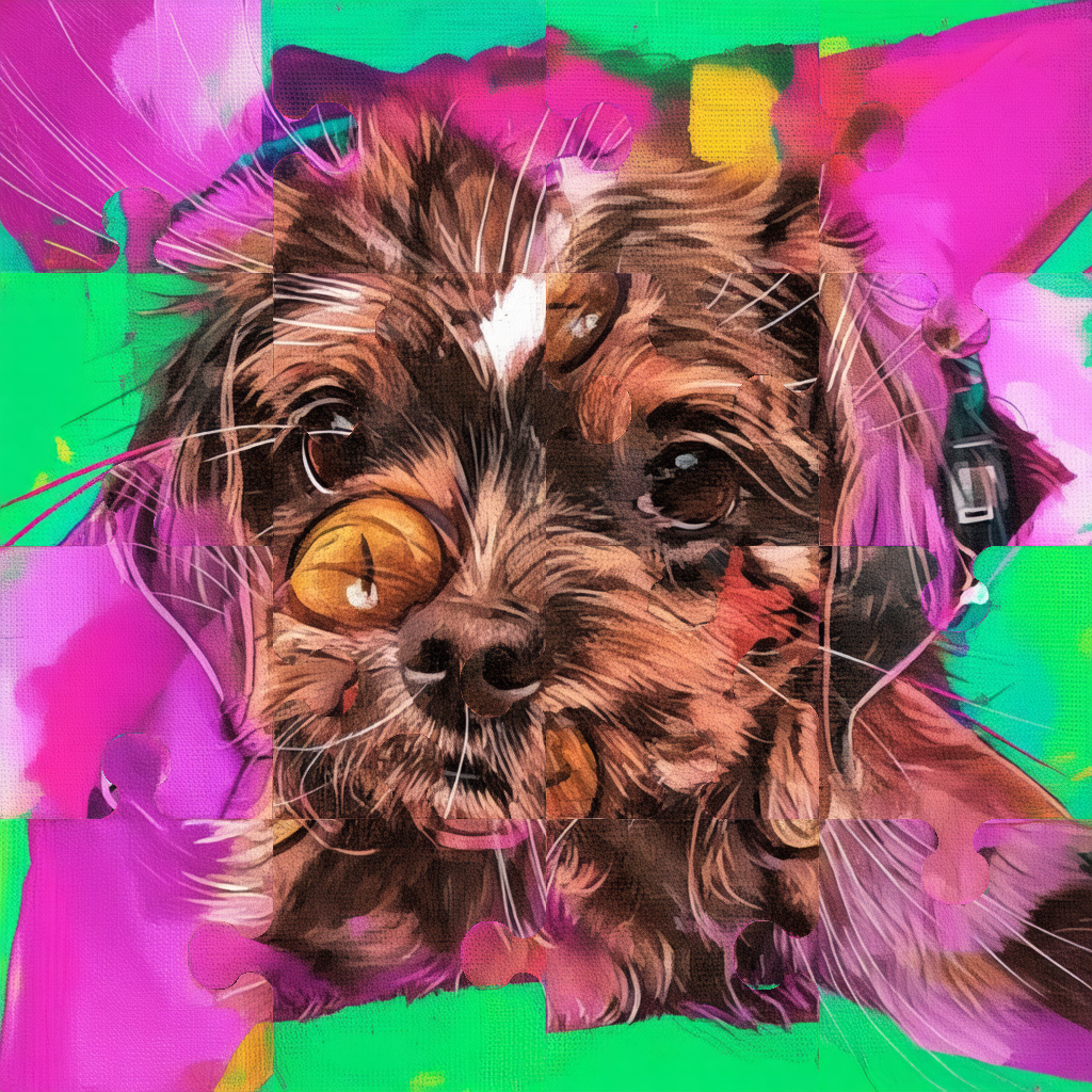
This project implements 2D latent generative anamorphoses using Stable Diffusion 3.5, inspired by LookingGlass (CVPR 2025). It generates a single image that reveals different content when viewed through simple geometric transformations, such as rotation, flipping, or jigsaw permutations.
Overview
The method creates a single anamorphic image that contains two prompts:
- View 1: The image as generated.
- View 2: The image after applying a specific transform (rotation, flip, or jigsaw).
Supported 2D transforms:
- Rotations: 90°, 135°, 180° circular rotations
- Flips: Vertical and horizontal flips
- Jigsaw: Tile permutations inspired by Visual Anagrams
How It Works
We build on the diffusers library and modify the SD3.5 pipeline. The pipeline blends two diffusion trajectories using Laplacian Pyramid Warping. The core idea of the paper is to predict the clean latents in one scheduler step at each time step to get a solid estimate of all the \(N\) clean latents, decode them into the image space and then blend them in order to blend multiple view transformations. These are then rencoded to latents to perform the denoising step and move closer to the final clean image from time step 0 to \(T\). Noteably, Visual Anagrams (CVPR2024) opts to use pixel space models in order to avoid the difficulities of latent diffusion models.
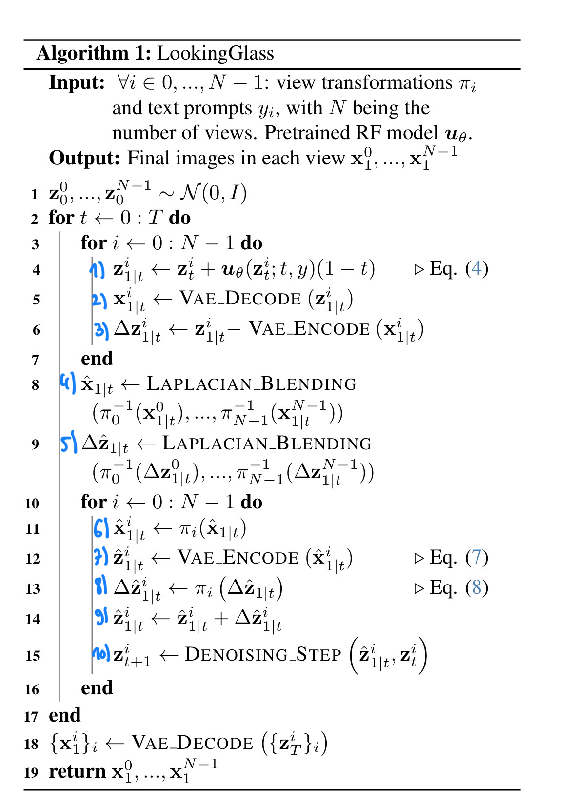
The algorithm from the paper is shown below, the “clean” predicted latents \(z_{1\vert t}^{i}\) of each view \(i\) are first predicted (step 1) in one single step and then decoded into the image space \(x_{1\vert t}^{i}\) with the VAE (step 2). Due to the fact that the decoding/encoding of the vae is lossy, a residual correction term \(\Delta\) \(z_{1\vert t}^{i}\) is introduced in step 3. Afterwards the predicted clean images are blended to obtain \(\hat{x}_{1\vert t}\) via Laplacian Pyramid Blending (step 4), similarly the residual correction factors are blended (step 5) to calculate \(\Delta\) \(\hat{z}_{1\vert t}\). During the blending step, tshe second view is transformed according to the specified view transform \(\pi^{-1}\).
After blending the views together, the view transform of the transformed image \(\hat{x}_{1\vert t}^{i}\) and residual correction \(\Delta\) \(\hat{z}_{1\vert t}^{i}\) are then obtained by inverting the view blended terms with \(\pi\) (step 6 and 8). In our implementation the first image undergoes no transform, so this step is only applied for the second image \(i=1\). Each image is then encoded back to its latent space \(\hat{z}_{1\vert t}^{i}\) (step 7) by encoding with the VAE. The latent correction of \(\hat{z}_{1\vert t}^{i}\) is then performed (step 9) before running the denoising (step 10) step.
While it may not be directly clear, the denoising step takes as input the current latent (from step 9) \(\hat{z}_{1\vert t}^{i}\) and latent of the previous timestep \(z_{t}^{i}\) (which corresponds to a one step clean latent prediction of the past step). So it is essentially an interpolation between the two latent spaces which can be implemented simply as such:
\(z_{t+1}^{i} = z_{t}^{i} + \frac{\sigma_{t+1}}{\sigma_{t}} \left(\hat{z}_{1\vert t}^{i} - z_{t}^{i}\right).\)
We can derive this from the rectified flow matching equation.
Deriving the interpolation
The current latent at noise level \(\sigma_{t}\) is \(z_{t}^{i} = (1 - \sigma_{t}) \, z_{0}^{i} + \sigma_{t} \, \epsilon.\)
From this, the direction from clean to current is \(z_{t}^{i} - z_{0}^{i} = \sigma_{t}(\epsilon - z_{0}^{i}).\)
The target latent at \(\sigma_{t+1}\) is \(z_{t+1}^{i} = (1 - \sigma_{t+1}) \, z_{0}^{i} + \sigma_{t+1} \, \epsilon.\)
Subtracting \(z_{0}^{i}\) gives \(z_{t+1}^{i} - z_{0}^{i} = \sigma_{t+1}(\epsilon - z_{0}^{i}) = \frac{\sigma_{t+1}}{\sigma_{t}} \left(z_{t}^{i} - z_{0}^{i}\right).\)
Rewriting, \(z_{t+1}^{i} = z_{0}^{i} + \frac{\sigma_{t+1}}{\sigma_{t}} \left(z_{t}^{i} - z_{0}^{i}\right).\)
Substituting \(z_{0}^{i}\) for \(\hat{z}_{1\vert t}^{i}\) results in the update above.
Examples
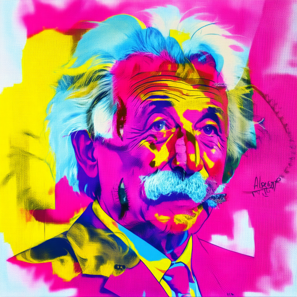
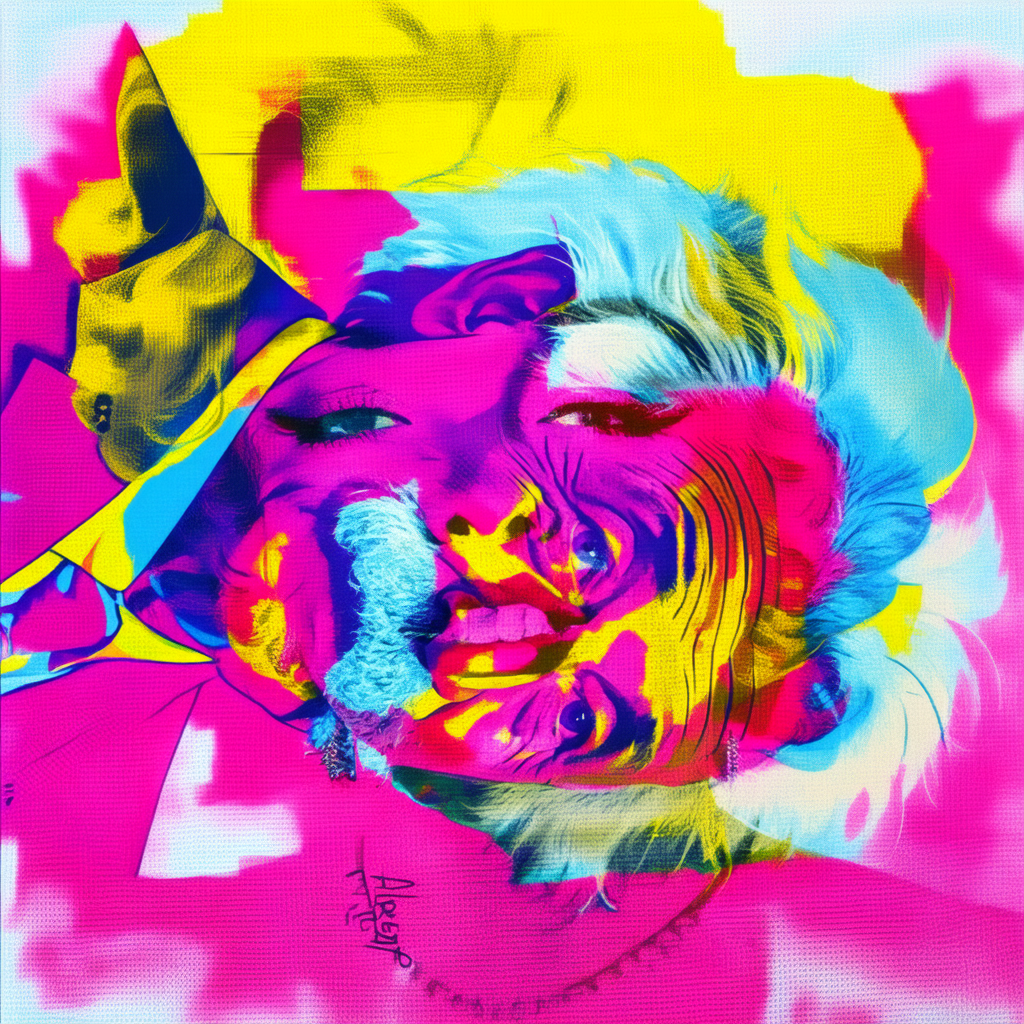
90° Rotation: Einstein ↔ Marilyn (Pop Art)
- Style prompt: “a pop art of”
- Prompt 1: “albert einstein”
- Prompt 2: “marilyn monroe”
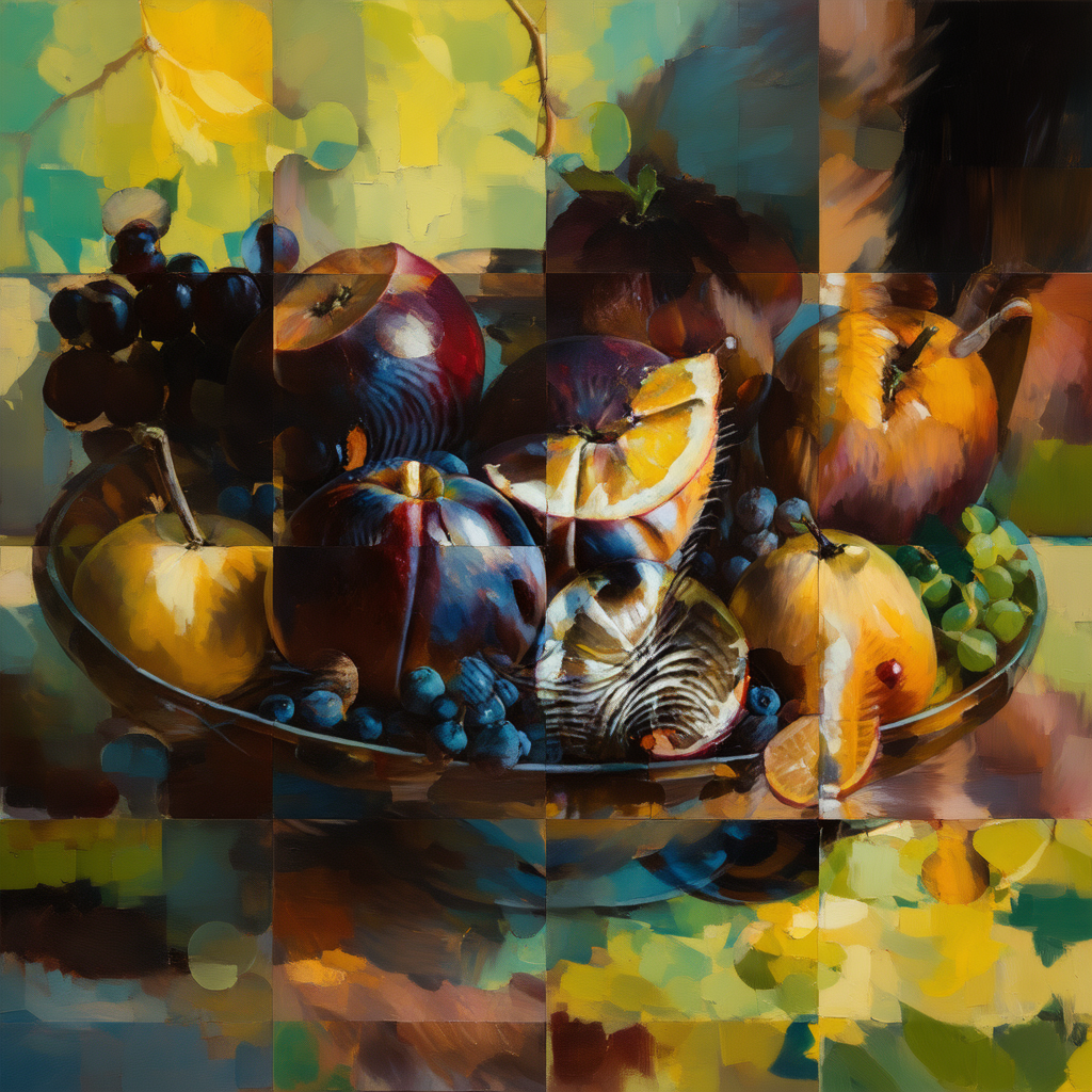
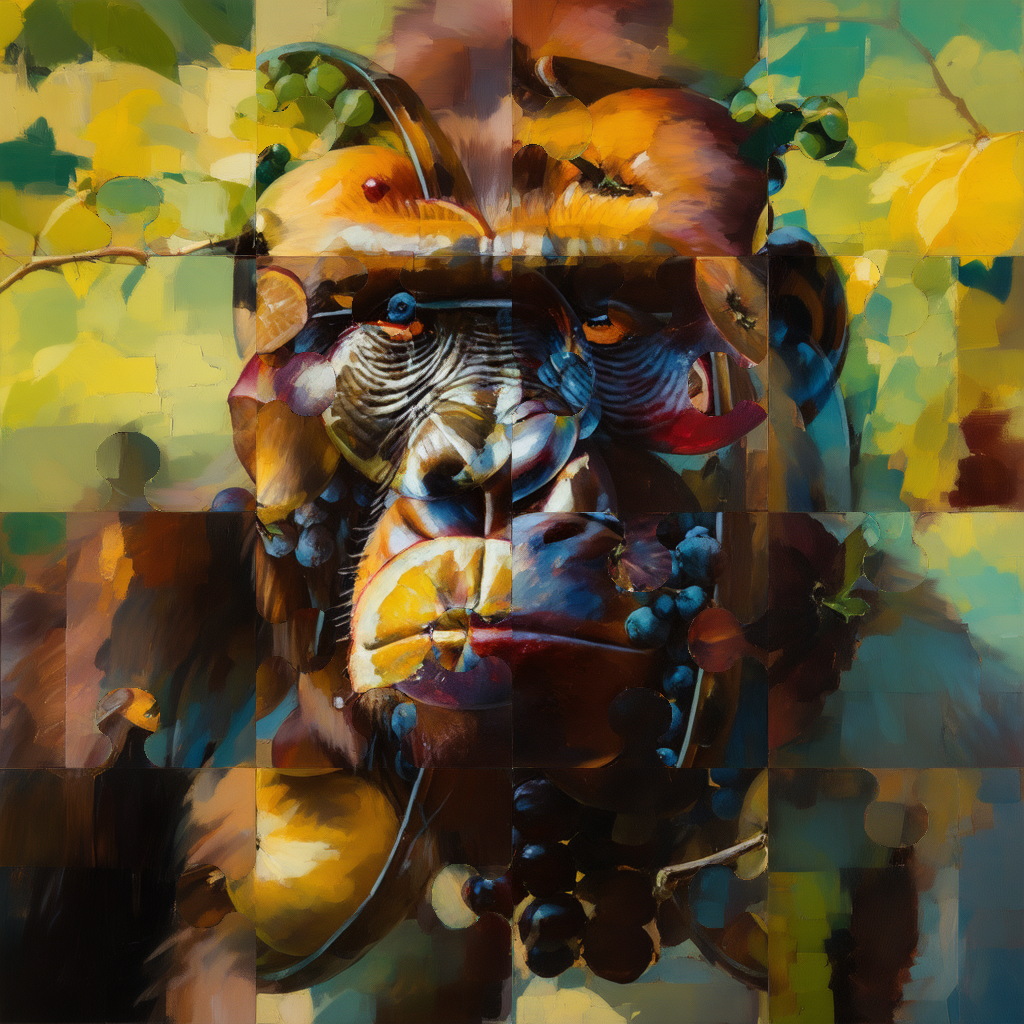
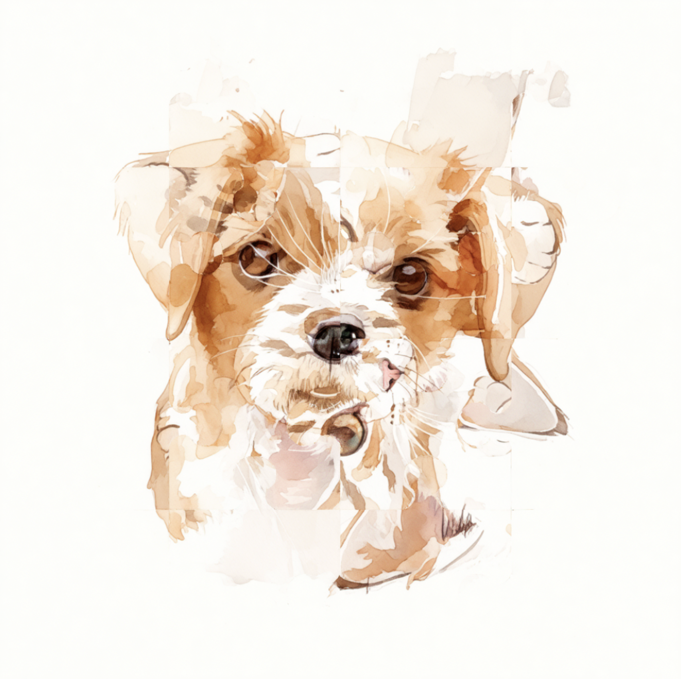
Jigsaw Transform: Fruit Bowl ↔ Gorilla
- Style prompt: “an oil painting of”
- Prompt 1: “a bowl of fruits”
- Prompt 2: “a gorilla”
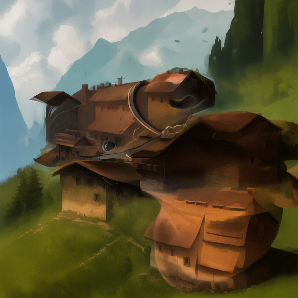
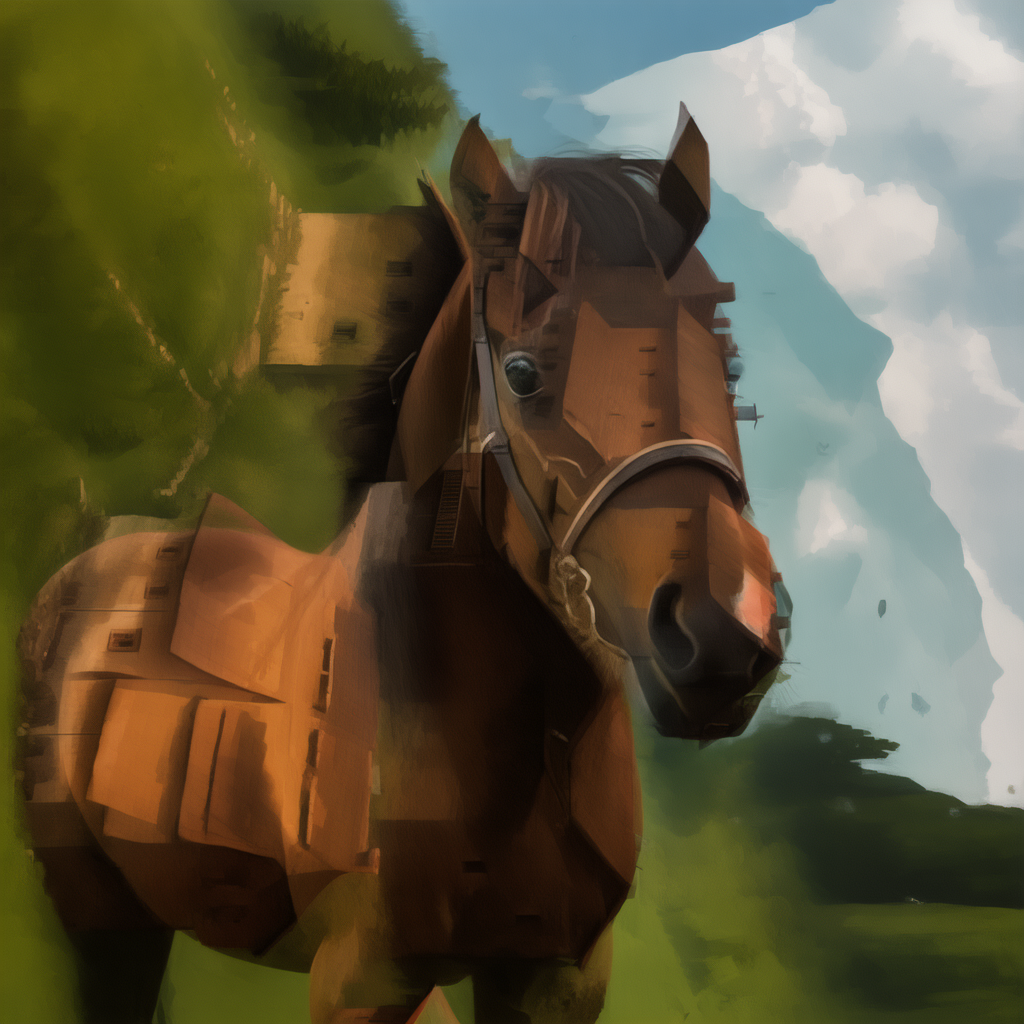
90° Rotation: Village ↔ Horse
- Style prompt: “a painting of”
- Prompt 1: “a village”
- Prompt 2: “a horse”
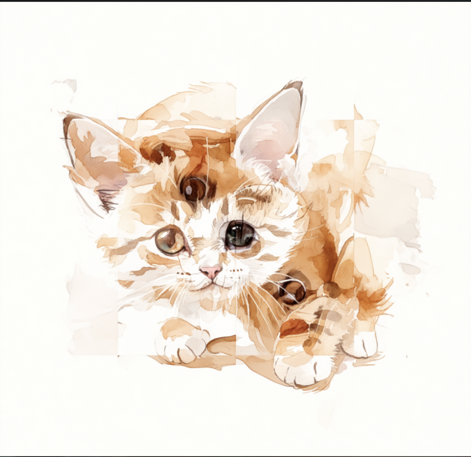
Jigsaw Transform: Puppy ↔ Cat
- Style prompt: “a water color painting of”
- Prompt 1: “a puppy”
- Prompt 2: “a cat”
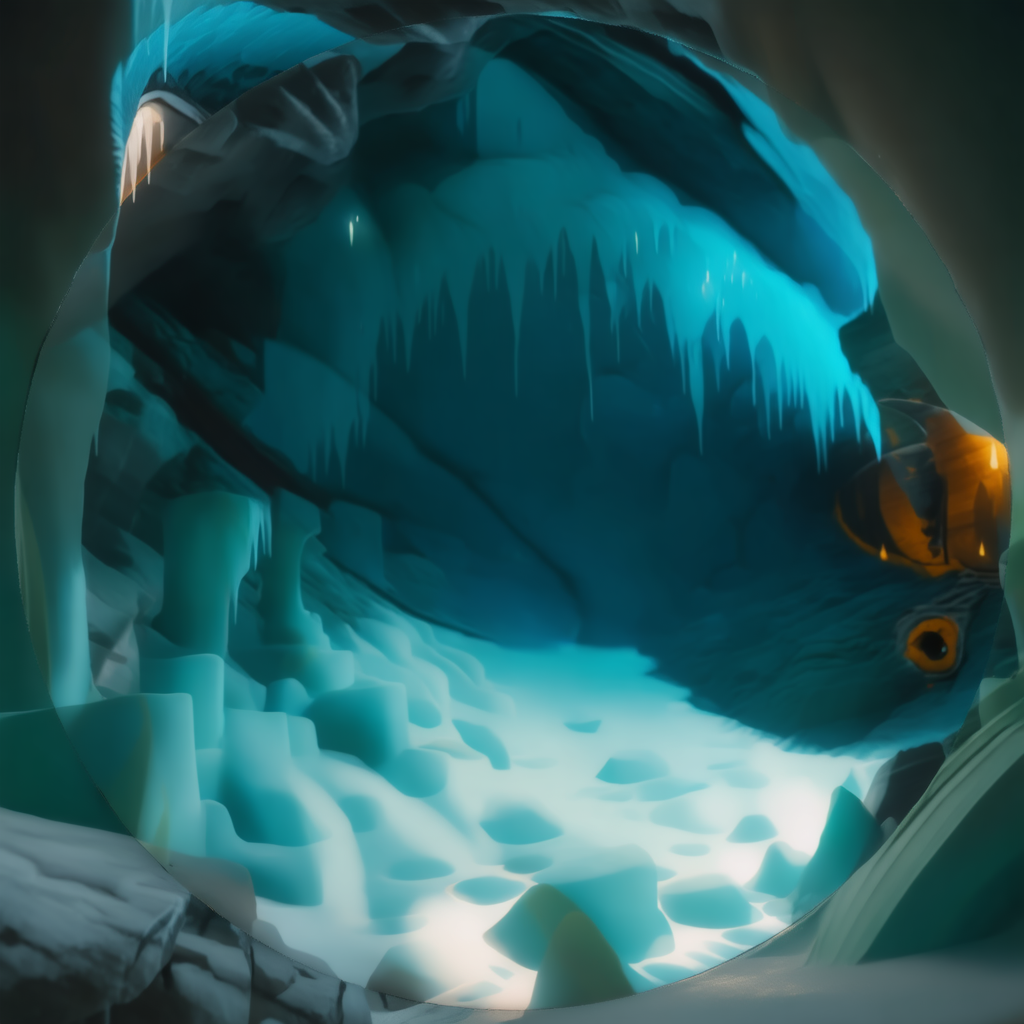
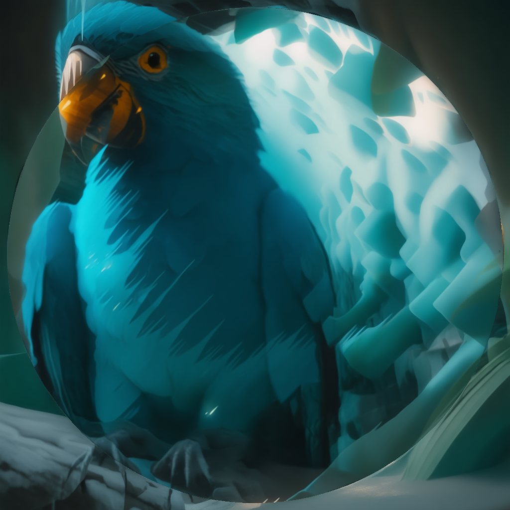
90° Inner Circular Transform: Cave ↔ Parrot
- Style prompt: “a rendering of”
- Prompt 1: “an icy cave”
- Prompt 2: “a parrot”
Repository
Project code: LatentGenerativeAnamorphoses
References
- Chang, Pascal, et al. “LookingGlass: Generative Anamorphoses via Laplacian Pyramid Warping.” Proceedings of the IEEE/CVF Conference on Computer Vision and Pattern Recognition, 2025, pp. 24-33.
- Geng, Daniel, Inbum Park, and Andrew Owens. “Visual Anagrams: Generating Multi-View Optical Illusions with Diffusion Models.” Proceedings of the IEEE/CVF Conference on Computer Vision and Pattern Recognition, 2024, pp. 24154-24163.