Summary Gradient Descent Optimization Algorithms
All you need is a good init suggests a novel initialization technique that allows the initalization of deep architectures wrt to other activations than ReLU (focus of Kaiming init)


- What did the authors want to achieve ?
- Key elements (Methods in this case)
- SGD Based
- Gradient descent optimization algorithms
- Results and Conclusion
What did the authors want to achieve ?
- give an overview of the different optimizers that exist and the challenges faced
- analyze additional methods that can be used to improve gradient descent
- the paper is more geared towards the mathematical understandinf of these optimizers as it does not make performance comparisons
Key elements (Methods in this case)
In the following all sorts of SGD variants and optimization algorithms will be adressed. The following parameters are universal in the upcoming formulas:
θ : parameters
η : learning rate
J(θ) : objective function depening on models parameters
SGD Based
Batch Gradient Descent
Formula :
$θ = θ − η · ∇θJ(θ)$
Code :
for i in range ( nb_epochs ):
params_grad = evaluate_gradient ( loss_function , data , params )
params = params - learning_rate * params_grad
This is the vanilla version, it updates all parameters in one update. It is redundant and very slow and can be impossible to compute for large datasets due to memory limitations. It also does not allow for online training.
Stochastic Gradient Descent (SGD)
SGD performs a parameter update for each training example ${x^i}$ and ${y^i}$ respectively and therefore allows online training as well as faster training and the ability to train larger datasets.
Formula :
$θ = θ − η · ∇θJ(θ; {x^i};{y^i})$
Code :
for i in range ( nb_epochs ):
np . random . shuffle ( data )
for example in data :
params_grad = evaluate_gradient ( loss_function , example , params )
params = params - learning_rate * params_grad
SGD also has the potential to reach better local minima, convergance is compilcated however but can be combated with weight decay,almost certainly converging to a local or the global minimum for non-convex and convex optimization respectively. As is common for most batch gradient descent techniques the data is also shuffled in the beginning, the advantages of shuffling are discussed in the additional strategies section.
Mini-Batch Gradient Descent (most commonly refered to as the actual SGD)
Mini-Batch Gradient Descent takes the best of both worlds and performs updates on smaller batches (common sizes range between 16 and 1024).
Formula :
$θ = θ − η · ∇θJ(θ; {x^{i:i+n}};{y^{i:i+n}})$
Code :
for i in range ( nb_epochs ):
np . random . shuffle ( data )
for batch in get_batches ( data , batch_size =50):
params_grad = evaluate_gradient ( loss_function , batch , params )
params = params - learning_rate * params_grad
It is usually refered to as SGD. This technique reduces the variance, which leads to better convergence. It can also make use of highly computationally optimized matrix operations to make computing the gradient of a mini-batch very fast.
Challenges of SGD
Vanilla SGD does not guarantee good convergence, so the following challenges have to be adressed :
- choosing the learning rate is very difficult, small values can lead to very slow convergence while large ones can lead to divergence
- techniques that combat this like annealing and scheduling of the $\eta$ are used to combat this, however they do not adjust to the dataset used and have to be specified in advance
- the learning rate is fixed for all parameters, however we would like to updates each parameter depending on the occurence of features (e.g. higher lr for rarer features)
- minimizing non-convex functions, where the convex criterion :
$f(\lambda*x_{1}+(1-\lambda)*x_{2}) {\leq } \lambda*f(x_{1}) + (1-\lambda) * f(x_{2})$
is not fullfilled, often leads to convergence in local minima. Often this is due to saddle points as Dauphin et al. found out.
Gradient descent optimization algorithms
In the following widely used optimization algorithms will be adressed. The following parameters are universal in the upcoming formulas:
θ : parameters
η : learning rate
J(θ) : objective function depening on models parameters
$γ$ : fraction that was introduced with Momentum (usually set to 0.9)
$t$ (index) : time step
$\epsilon$ : smoothing term to avoid division by zero, introduced by Adagrad (usuall set to 1e-8)
Momentum
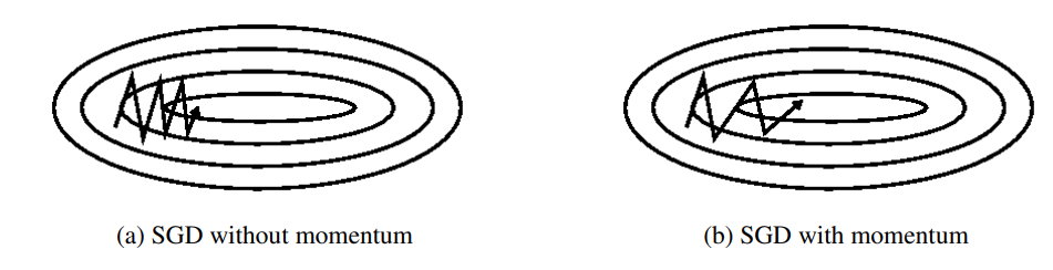
SGD has trouble navigating ravines (area where surface curves much more steeply in one dimension than in another), SGD often oscillates in these cases while only making small progress. These are common around local optima.
Momentum helps accelerate SGD in the relevant direction and dampens these ocsillations by introducing a new $γ$ term that is used to add a fraction of the update vector of the past time step to the current update vector.
Formula :
$vt = γv_{t−1} + η∇θJ(θ)$
$θ = θ − v_{t}$
An analogy to this is a ball rolling dowhill, it becomes faster on the way (until it reaches its maximum speed due to air resistance, i.e. $γ<1$)
Nesterov accelerated gradient (NGA)
The idea of NGA is that we do not want to blindly go downhill, but rather know when the uphill section starts so we can slow down again. NGA does take this into account by using our momentum term $γv_{t−1}$ to approximate the next time step using $θ − γv_{t}$. (only the gradient is missing for the full update). This allows us to compute the gradient w.r.t the approximate future position of our parameters rather than the current one.
Formula
$vt = γv_{t−1} + η∇θJ(θ-γv_{t−1})$
$θ = θ − v_{t}$
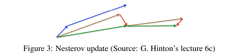 NAG first makes a jump in the direction of calculated gradient (brown vector) and then makes a correction (green vector)
This anticipatory update prevents us from going too fast and results in increased
responsiveness, which has significantly increased the performance of RNNs on a number of tasks. Now we are able to update e
NAG first makes a jump in the direction of calculated gradient (brown vector) and then makes a correction (green vector)
This anticipatory update prevents us from going too fast and results in increased
responsiveness, which has significantly increased the performance of RNNs on a number of tasks. Now we are able to update e
Results and Conclusion
The authors were able to give a good overview of different SGD techniques and it's optimizers like Momentum, Nesterov accelerated gradient, Adagrad, Adadelta, RMSprop, Adam, AdaMax, Nadam, as well as different algorithms to optimize asynchronous SGD. Additionally strategies that can improve upon this like curriculum learning, batch norm and early stopping were deployed.