Summary Mixup Augmentation Technique
Suggests a multi class augmentation technique to improve generalization, memorization of corrupted labels and improves robustness against adversarial examples


Problems of existing rechniques :
- ERM memorizes, does not generalize -> vulnerable to adversarials
- Classic data augmentation is used to define neighbors in a single class, this is mostly hand crafted by humans and does not consider multi class combinations ## What did the authors want to achieve ?
- improve on undesirable memorization of corrupted labels and sensitivity to adversarial examples
- stabilize training (especially of GANs)
Key elements
The Expected Risk (ER), assuming that the joint distribution between a random input $X$ and a label $Y$ $P(X,Y)$ is an empirical distribution :
$P_{\delta}(x,y) = \frac{1}{n}\sum_{i=1}^{n}\delta(x=x_{i},y=y_{i})$
We can infer the approximation of the expected risk $R_{\delta}(f)$ since $dP_{\delta}(x,y) = 1$, and the loss $l(f(x),y) = \sum_{i=1}^{n}l(f(x_{i}),y_{i})$ :
$R_{\delta}(f) = \int l(f(x),y)*dP_{\delta}(x,y)=\sum_{i=1}^{n}l(f(x_{i}),y_{i})$
The Empirical Risk Minimization (ERM) (Vapnik,1998) is known as learning our function $f$ by minimizing the loss. $P_{\delta}$ is a naive estimation as it is one of many possible choices. The paper also mentions Vicinal Risk Minimization (Chapelle et al., 2000) which assumes the distribution P to be a sum of all the inputs and labels over a vicinity distribution $v(\tilde{x},\tilde{y}|x_{i},y_{i})$ and measures the probability of finding the virtual feature target pair $(\tilde{x},\tilde{y})$ in the vicinity of the training feature-target pair $(x_{i},y_{i})$. The approach considered Gaussian vicinities, which is equal to augmenting the training data with additive Gaussian noise. Considering a Dataset of size m, we can infer the empirical vicinal risk :
$R_{v}(f) = \frac{1}{m}\sum_{i=1}^{m}l(f(\tilde{(x_{i}}),\tilde{y_{i}})$
This paper introduces a different generic vicinal distribution, called mixup :
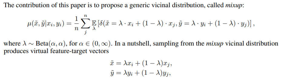
With $\lambda = [0,1]$ and $(\tilde{x_{i}},\tilde{y_{i}})$ & $(\tilde{x_{j}},\tilde{y_{j}}) being 2 random target vectors$. The mixup parameter $\alpha$ controls the strength of interpolation between the pair, as $\alpha \rightarrow 0$ it increasingly recovers to the ERM principle.
The implementation from the paper is relatively straightforward :
for (x1, y1), (x2, y2) in zip(loader1, loader2):
lam = numpy.random.beta(alpha, alpha)
x = Variable(lam * x1 + (1. - lam) * x2)
y = Variable(lam * y1 + (1. - lam) * y2)
optimizer.zero_grad()
loss(net(x), y).backward()
optimizer.step()
What does it do ? Mixup makes the model behave linearly in-between classes/examples, this reduces the amount of oscillations when facing a new example that is outside of the training examples. This happens linearily and is simple and therefore a good bias from the Occam's razor point of view ( "Entities should not be multiplied without necessity.").
Results and Conclusion
The authors prove that mixup is a very effective technique across all domains.
Classification
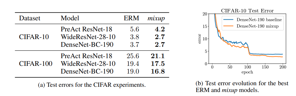 Experiments were made on both ImageNet and CIFAR-10/100 using different alphas for each dataset. $\alpha[0.1,0.4]$ for ImageNet and $\alpha = 1$ for CIFAR-10/100. Comparisons were made using different DenseNet and ResNet models. You can refer to the paper for the exact hyperparameters used in each case. As we can see in the graph above, miuxp outperforms their non-mixup counterparts. Learning rate decays were used @ epochs 10/60/120/180 with an inital value of 0.1 and training was done for a total of 300 epochs.
Speech Data
The google command dataset was used which contains 30 classes of 65000 examples. LeNet and VGG-11 were used with ADAM and a learning rate of 0.001 and mixup variants with alphas of 0.1 and 0.2 were compared to the ERM counterparts. Mixup was able to outperform ERM with VGG-11 which had the lowest error of all models (3.9 percent) on the validation set. LeNet however performed better without mixup applied. Comparing these outcomes, the authors infer that mixuxp works particularly well with higher capacity models.
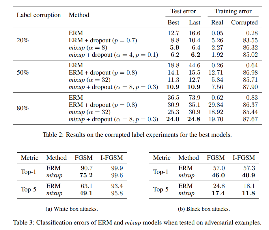
Memorization of corrupted labels (Table 2)
Robustness to corrupted labels is compared to ERM and mixup. An updated version of CIFAR is used where 20%,50% and then 80% are replaced by random noise. Usually Dropout was considered to be the best technique for corrupted label learning, so dropout with p ∈ {0.5, 0.7, 0.8, 0.9} and mixup are compared to each other along with a combo of both where α ∈ {1, 2, 4, 8} and p ∈ {0.3, 0.5, 0.7}. The PreAct ResNet-18 (He et al., 2016) model implemented in (Liu, 2017) was used. The model was trained for 200 epochs.
Robustness to adversarial example (Table 3)
Several methods were proposed, such as penalizing the norm of the Jacobian of the model to control the Lipschitz constand of it. Other approaches perform data augmentation on adversarial examples. All of these methods add a lot of compute overhead to ERM. Here the authors prove that mixup can improve on ERM significantly without adding significant compute overhead by penalizing the norm of the gradient of the loss wrt a given input along the most plausible directions (the directions of other training points). ResNet101 models were trained 2 models were trained on ImageNet with ERM and one was trained with mixup. White box attacks are tested at first . For that, the model itself is used to generate adversarial examples fusing FGSM or iterative FGSM methods, 10 iterations with equal step sizes are used, $\epsilon=4$ was set as maximum perturbation for each pixel. Secondly black box attacks are done, this is achieved by using the first ERM model to produce adversarials with FGSM and I-FGSM. Then the robustness of the second ERM model and the mixp model to these exampels is tested.
As we can see in table 3, mixup outperforms ERM in both cases significantly, being p to 2.7 times better when it comes to Top-1 error in the FGSM white box attack category.
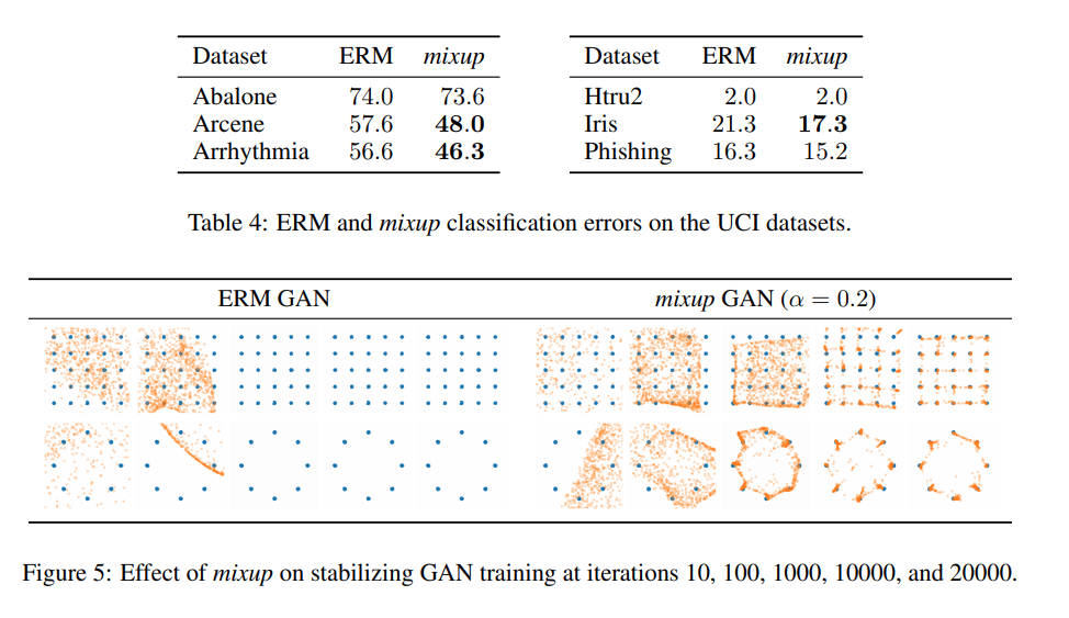
Tabular Data (Table 4)
A series of experiments was performed on the UCI dataset. A FCN with 2 hidden layers & 128 ReLU units was trained for 10 epochs with Adam and a batch size of 16. Table 4 shows that mixup improves test error significantly.
Stabilize GAN Training (Table 5)
When training GANs, the mathematical goal is to solve the optimization problem :
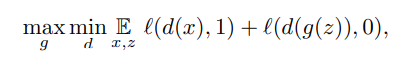
the binary cross entropy loss is used in this case. Solving this equation is a very difficult optimization problem (Goodfellow et al., 2016) as the discriminator often provides the generator with vanishing gradients. Using mixup, the optimization problem looks like this :
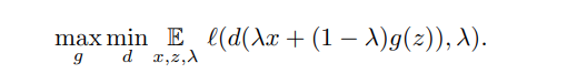
The models are fully connected, with 3 hidden layers and 512 ReLU units. The generator accepts 2D Gaussian noise vectors, 20000 mini-batches of size 128 are used for training with the discriminator being trained for 5 epochs before every generator iteration. Table 5 shows the improved performance of mixup.
A part of these mostly supervised use cases (except for GANs), the authors believe that other non straightforward use cases such as segmentation or different unsupervised techniques should be promising areas of future research.