Summary Bag of Tricks for Image Classification with Convolutional Neural Networks
Suggesting model refinements and architecture improvements to improve upon existing architectures and accelerate training time.
Key elements
Training Loop pseudocode :
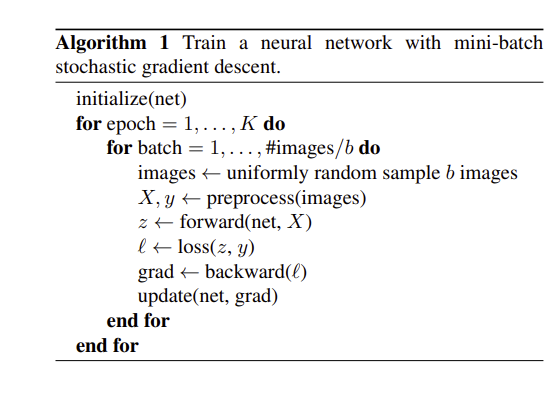
Training
-
The training/model builds on a "vanilla" training loop above, the ResNet architecture which is then improved, starting with these steps :
1) decode random image to FP32 in a range from [0,255]
2) crop random area with between [8%,100%] of total pixels and a of ration $4/3$ or $3/4$, then rescale to 224x224
3) flip horizontally with probability of 0.5
4) scale hue, saturation and brightness by randomly drawing from [0.6,1.4]
5) Add PCA Noise w/coefficient randomly sampled from ~ $N(0,0.1)$
6) normalize RGB : substract 123.68/116.779/103.939 and divide by 58.393/57.12/57.375
The CNN is initalized using Xavier Init and uniformally initalizing the weights from [-a,a] with $a =\sqrt{6 / (d_{in} + d_{out})}$ with the two $d$ values corresponding ti input and output filter size. Biases are initalized to 0 as well the Batch Norm vector $\beta $, $\gamma$ vectors are initalized to 1. Nesterov acclerated Momentum is used with 120 epochs and a total batch size of 256, the learning rate is initalized to 0.1 and cut by 10 at the 30th, 60th and 90th epoch.
Large Batch Size, linear scaling learning rate
In the past using large Batch sizes has been difficult (degradation), as larger batch sizes posses less noise, the variance is smaller than on small batch sizes. 4 tricks improve upon this problem :
Linear Scaling Learning Rate :
- Linear scaling learning rate was proposed by Goyal et. al, the paper proposes that linear scaling the learning rate with batch size empirically improves ResNet training. He et. al built on this and chooses 0.1 as initial learning rate for batch size of 256. Assuming our batch size is $b$ we scale like this :
$0.1 * b/256$
Learning Rate Warmup :
- at the beginning all parameters are typically random values, therfore large learning rates can lead to numerical instability.Goyal et. al proposes a gradual learning rate increase to combat this. For that $m$ warmup epochs are selected, if our inital learning rate is $\eta$, our value depending on epoch $i$ is :
$i*\eta/(m)$
Zero $\gamma$:
- Residual Blocks can consist of Batch Norm layers at the output. Initalizing the $\gamma$ parameters of the Batch Norm layers to 0, mimics smaller networks which makes the parameters easier to initalize. That is achieved because when using 0 for intialization only the input (shortcut connection that is passed to the end of the block) is learned when both $\gamma$ and $\beta$ are zero at the inital stage.
No bias decay :
- Weight decay is only applied to the weights and not the biases as well as the two Batch Norm hyperparamters, this avoids overfitting.
Low Precision Training
In order to improve training time (from 13.3 minutes w/ batch size of 256 per epoch to 4.4 minutes per epoch with batch size of 1024 for ResNet-50), FP16 is used to store activations and gradients, however copies are made in FP32 for parameter updates. Optionally multiplying a scalar to the loss can make up for the lower range of FP16.
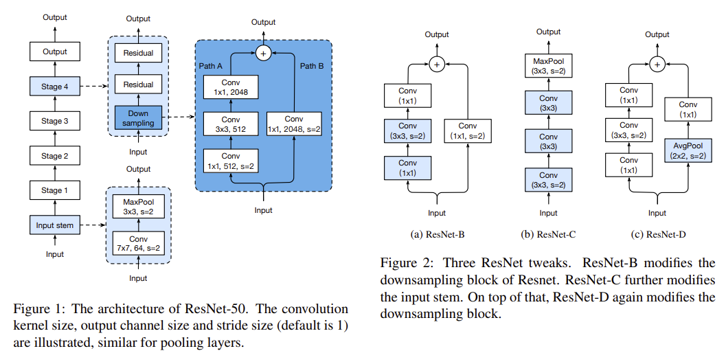
Over the year several improvements to the classic ResNet where introduced (picture above). The paper also introduces a new improvement.
Architecture Improvements
ResNet-B
Resnet-B researchers found out that "ResNet-A" (the original version) ignores three quarters of the input map, due to a 1x1 conv with a stride of 2 in the beginning. Due to that the researchers switched the stride of 2 between the first two layers in Path A.
ResNet-C
This version only changes the start of the network. The computation of a 7x7 Kernel Convolution is 5.4 times slower as a 3x3 vonvolution, that's why the 7x7 Kernel with stride 2 was replaced with 3x3 Kernels (the first two are with 32 filters and stride of 2/1, while the last one has 64 filters and stride of 1).
ResNet-D
The approach proposed in the paper focuses on the same approach as the ResNet-B researchers did, but in this case Path B is changed. Path B also ignores 3/4 of input due to a 1x1 convolution used at the start of Path B. The paper implements an average Pooling Layer of size 2x2 with stride of 2, before the convolution (now with stride 1). The compute cost is very small. Experiments show that, ResNet-D only needs 15% more compute with a 3% lower throughput than the vanilla architecture.
Training Refinements
Cosine Learning Rate Decay
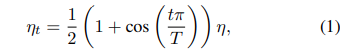
Cosine annealing (1) is used to decay the learning rate (compared to divsion by 10 every 30 epochs in He et. al). $T$ is the total number of batches. Compared to the step decay, the cosine decay starts to decay the learning since the beginning, but remains large until step decay reduces the learning rate by 10x, which potentially improves the training progress.
Label Smoothing
During training we are minimzing Cross Entropy Loss :
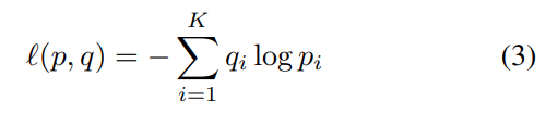
, where $q_{i}$ is the Softmax output
Looking at the loss (refer to the paper), it encourages scores to be dramtically distinctive from others. Therefore label smoothing was introduced with Inception-v2 :
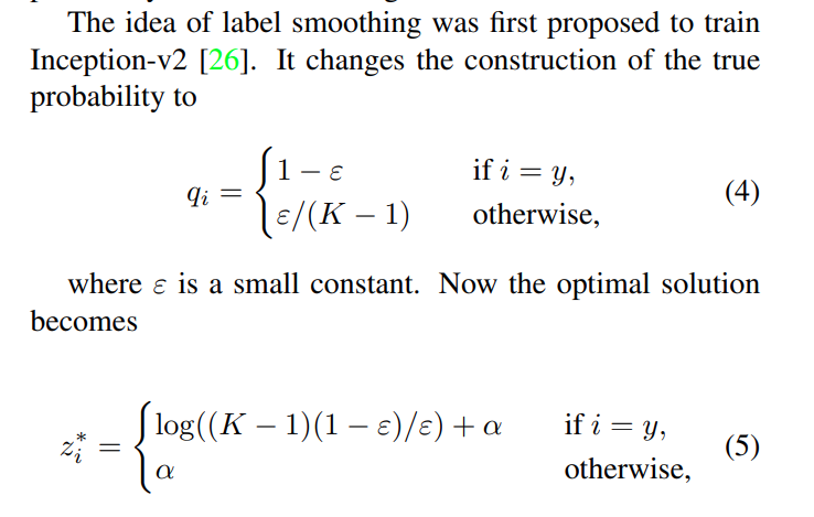
Which can generalize better, due to a finite output that is encouraged from the fully connected layer and can generalize better. In the experiments $\epsilon$ is set to 0.1 following Szegedy et al.
Knowledge Distillation
With this approach a pretrained teacher model, teaches a model that has to be trained still. For example a ResNet-152 teaches a ResNet-50. A distillation loss (negative Cross Entropy loss) is used to compare the two Softmax outputs. The total loss then changes to :
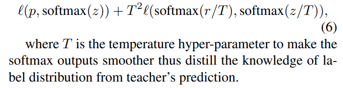 , where $p$ is the true probability distribution and $z$ and $r$ are the student and learner outputs. T is set 20 here, for a pretrained ResNet-152-D model with cosine decay and label smoothing applied.
Mixup Training
Mixup is another training refinement, according to Jeremy Howard from fastai it could be better than the other augmentation techniques and is also multidomain. Mixup samples 2 images in this case and interpolates between them (using weighted interpolation) :
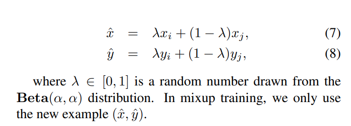
During the experiments $\alpha$ is set to 0.2 in the Beta Distribution. The # of epochs is increased from 120 to 200. Using mixup and distillation, the teacher model can be trained with mixup as well.
Results and Conclusions
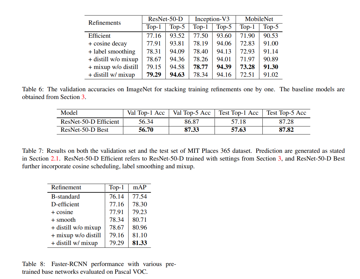
Results can be seen in the picture above.
FP16 further improves training by 0.5% and the ResNet-D approach improves accuracy by 1% over the standard approach.
Object Detection
A VGG-19 Faster-RCNN model is trained with Detectron refinements such as linear warmup and long training schedule. Using destill with mixup the mAP can be improved from 77.54 to 81.33.
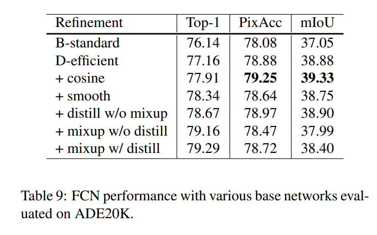
Semantic Segmentation
A FCN model is used pre trained on the ADE20K dataset. Both pixel accuracy and mean intersection over union improved.