Summary of the ResNet paper

• Summary of the ResNet paper
  • What did the authors want to achieve ?
  • Key elements
    • Residual Learning
    • Shortcuts
    • Deeper Bottleneck Architectures
    • Implementation Details
  • Implementation of a ResBlock
  • Results and Conclusion

Summary of the ResNet paper

The architecture that won the 1st place on the ILSVRC 2015 classification task.

What did the authors want to achieve ?

• Allow training of deep Networks
• Improve Computer Vision Performance, by enabling the use of deeper architectures as depth is of crucial importance (as can be seen with to other ImageNet winners) => This applies to different vision tasks
• Normalization and Initialization have largely adressed vanishing/exploding gradients in deep networks, however accuracy gets saturated and then degrates quickly with more depth :
  deep residual learning should help adress this issue and build on existing ideas such as shortcut connections

Key elements

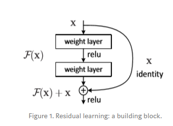
Residual Learning

• $H(X)$ is considered to be the mapping of a few stacked layers. The idea of Residual Blocks, is that this mapping function $H(x) = F(x) + x$ can more easily be learned when we let it approximate this Residual funciton. This is based on the degradation problem, which suggests that the solvers might have difficulties in approximating identity mappings by multiple nonlinear layers. The identity mapping should then allow deeper models to have an error no greater than that of a shallow counterpart. In reality, the identity mapping probably is not optimal, but it can still allow us to pre-condition the problem. This is shown by the small responese of the learned residual functions, which suggest that these mappings provide reasonable preconditioning. If the residual funciton has only a single layer, it resembles a linear function $y = W*x +x$, which is why an advantage can only be observed with more than one layer.

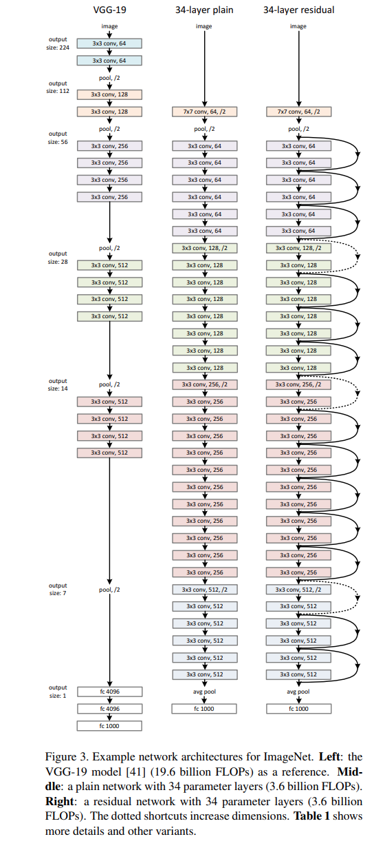
The comparison between a plain 34-layer and 34-layer residual network looks like this :

Shortcuts

3 different Shortcuts are used :

A) zero-padding shortcuts are used
for increasing dimensions, and all shortcuts are parameterfree
B) ) projection shortcuts are used for increasing dimensions, and other shortcuts are identity
C) all shortcuts are projections

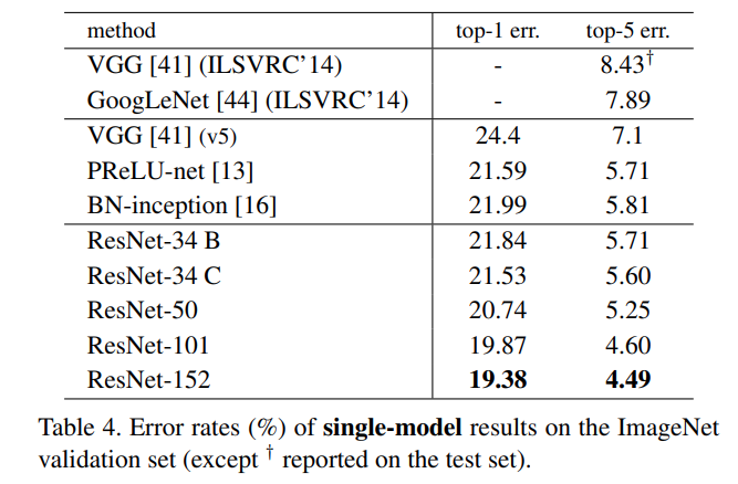
All 3 above are better than the plain counterpart, however C is slightly better than B, which is also slighlty better than A (see Table 4, under Classification). But the small differences are not essential for the degradation problem, and C adds parameters which has a negative impact on time/memory complexity.

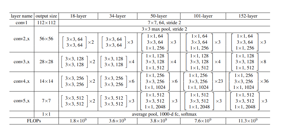
Deeper Bottleneck Architectures

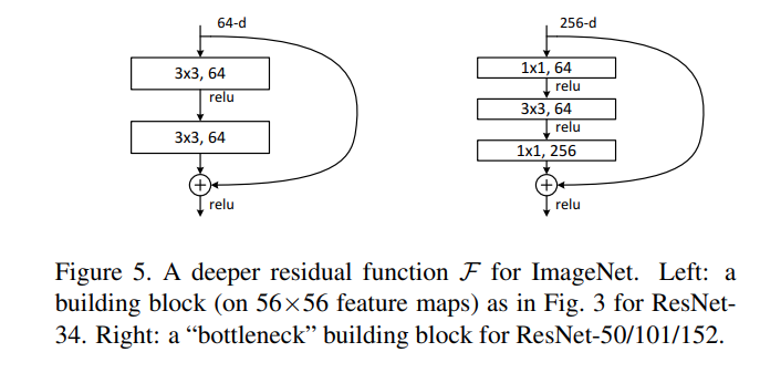Because of training time, the block is redesigned as a bottleneck with smaller I/O dimensions. The three layers are 1×1, 3×3, and 1×1 convolutions, where the 1×1 layers are responsible for reducing and then increasing (restoring) dimensions, leaving the 3×3 layer a bottleneck with smaller input/output dimensions. Identity shortcut connections are key, as with projection the model size and time complexity would double.

Implementation Details

• 224x224 random crop is randomly sampled from an image, horizontal flips are used
• SGD is used with lr starting at 0.1 and being divided by 10 as the error plateaus
• training for up to 60x1e5 iterations
• weight decay : 0.0001 and momentum of 0.9

Implementation of a ResBlock

A Residual Block can be implemented as follows in PyTorch :

def conv(in_channels, out_channels, kernel_size, stride=2, padding=1, batch_norm=True):
    """Creates a convolutional layer, with optional batch normalization.
    """
    layers = []
    conv_layer = nn.Conv2d(in_channels=in_channels, out_channels=out_channels,kernel_size=kernel_size, stride=stride, padding=padding,bias=False)

    layers.append(conv_layer)

    if batch_norm:
        layers.append(nn.BatchNorm2d(out_channels))
    return nn.Sequential(*layers)

class Resblock(nn.Module): 
    def __init__(self,conv_dim): 
        super(Resblock,self).__init__()
        self.conv1 = conv(conv_dim, conv_dim, kernel_size=3, stride=2, batch_norm=True)
        self.conv2 = conv(conv_dim, conv_dim, kernel_size=3, stride=2, batch_norm=True)
    def forward(self,x): 
        out1 = F.leaky_relu(self.conv1(x))
        out =  x + F.leaky_relu(self.conv2(out1))
        return out

def resblocks_create(conv_dim,n_res_blocks):
    res_layers = []
    for l in range(0,n_res_blocks):
        res_layers.append(Resblock(conv_dim))
    return nn.Sequential(*res_layers)

Instead of the conv function, you could obviously use the Impl

Results and Conclusion

Classification :

• the models are trained on the 1.28 million training images of ImageNet 2012. The 50k images val set and 100k images test set is used. At first Plain Networks are compared to it's respective ResNet with identity mapping and 0 padding, which does not add extra parameters. The results show that the degradation error is adressed better which allows better performance with increased depth and allowed them to win the ImageNet Challenge in 2015. The experiments show that depth matters as it allows lower classification error :
  

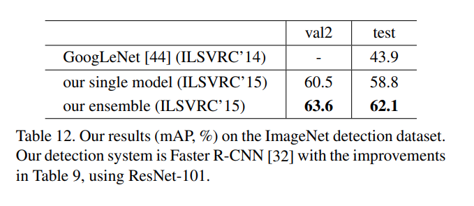
Object Detection :

• Faster R-CNN is used, but unlike VGG-16, no hidden layers are used. A full images shared feature map is computed, using layers whose stride on the image is not greater than 16 pixels. (i.e., conv1, conv2 x, conv3 x, and conv4 x, totally 91 conv layers in ResNet-101) These layers are anologous to VGG-16's 13 conv-layers and thereby have the same total stride (16 pixels). In consequence these layers are shared by a RPN with 300 proposals. . RoI pooling is performed before conv5_1. On this RoI-pooled feature, all layers of conv5 x and up are adopted for each region, playing the roles of VGG-16’s fc layers. Sibling layers (classification and bounding box regression) are used to replace the final classification layer. The BN layers are fixed, based on each layers Image Net mean and variance statistic. With this technique, using ResNet-101 the mAP (@0.5 IOU) can be improved a lot :

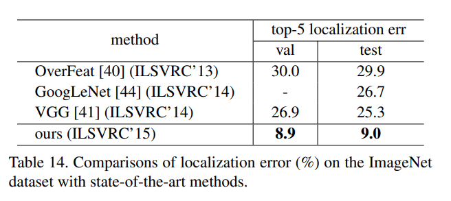
Object localization :

• a per class regression strategy is used (Bounding Box regressor for each class is learned). The Region Proposal Network ends with two sibling 1x1 convs for binary classification. So the Classification layer has a 1000 Dimension output, and for each dimension we predict if it is this object or not (binary). The regression layer has a 1000x4 d output, with box regressors for all 1000 classes based on multiple translation-invariant anchor boxes. Usually 8 acnhors are randomply sampled from the image, this avoids the dominance of negative samples. Data Augmentation is used, by sampling random 224x224 crops. Using ResNet-101 the state of the art can be improved :