Fastai Course DL from the Foundations Batch Norm
Implementing Batch Norm, Layer Norm, Instance Norm, Group Norm and running batch norm (Lesson 3 Part 4)


#collapse
%load_ext autoreload
%autoreload 2

%matplotlib inline
#collapse
from exp.nb_06 import *
Let's get the data and training interface from where we left in the last notebook.
#collapse
x_train,y_train,x_valid,y_valid = get_data()

x_train,x_valid = normalize_to(x_train,x_valid)
train_ds,valid_ds = Dataset(x_train, y_train),Dataset(x_valid, y_valid)

nh,bs = 50,512
c = y_train.max().item()+1
loss_func = F.cross_entropy

data = DataBunch(*get_dls(train_ds, valid_ds, bs), c)
#collapse
mnist_view = view_tfm(1,28,28)
cbfs = [Recorder,
        partial(AvgStatsCallback,accuracy),
        CudaCallback,
        partial(BatchTransformXCallback, mnist_view)]
#collapse
nfs = [8,16,32,64,64]
#collapse
learn,run = get_learn_run(nfs, data, 0.4, conv_layer, cbs=cbfs)
#collapse
%time run.fit(2, learn)
Let's start by building our own BatchNorm layer from scratch. We should be able to improve performance a lot. While training we keep a running exponentially weighted mean and variance average in the update_stats function. During inference we only use running mean and variance that we keep track off. We use register_bufferto create vars and means, this still creates self.vars and self.means, but if the model is moved to the GPU so will all buffers. Also it will be saved along with everything else in the model.
#collapse_show
class BatchNorm(nn.Module):
    def __init__(self, nf, mom=0.1, eps=1e-5):
        super().__init__()
        # NB: pytorch bn mom is opposite of what you'd expect
        self.mom,self.eps = mom,eps
        self.mults = nn.Parameter(torch.ones (nf,1,1))
        self.adds  = nn.Parameter(torch.zeros(nf,1,1))
        self.register_buffer('vars',  torch.ones(1,nf,1,1))
        self.register_buffer('means', torch.zeros(1,nf,1,1))

    def update_stats(self, x):
        #we average over all batches (0) and over x,y(2,3) coordinates (each filter)
        #keepdim=True means we can still broadcast nicely as these dimensions will be left empty
        m = x.mean((0,2,3), keepdim=True)
        v = x.var ((0,2,3), keepdim=True)
        self.means.lerp_(m, self.mom)
        self.vars.lerp_ (v, self.mom)
        return m,v

    def forward(self, x):
        if self.training:
            with torch.no_grad(): m,v = self.update_stats(x)
        else: m,v = self.means,self.vars
        x = (x-m) / (v+self.eps).sqrt()
        return x*self.mults + self.adds
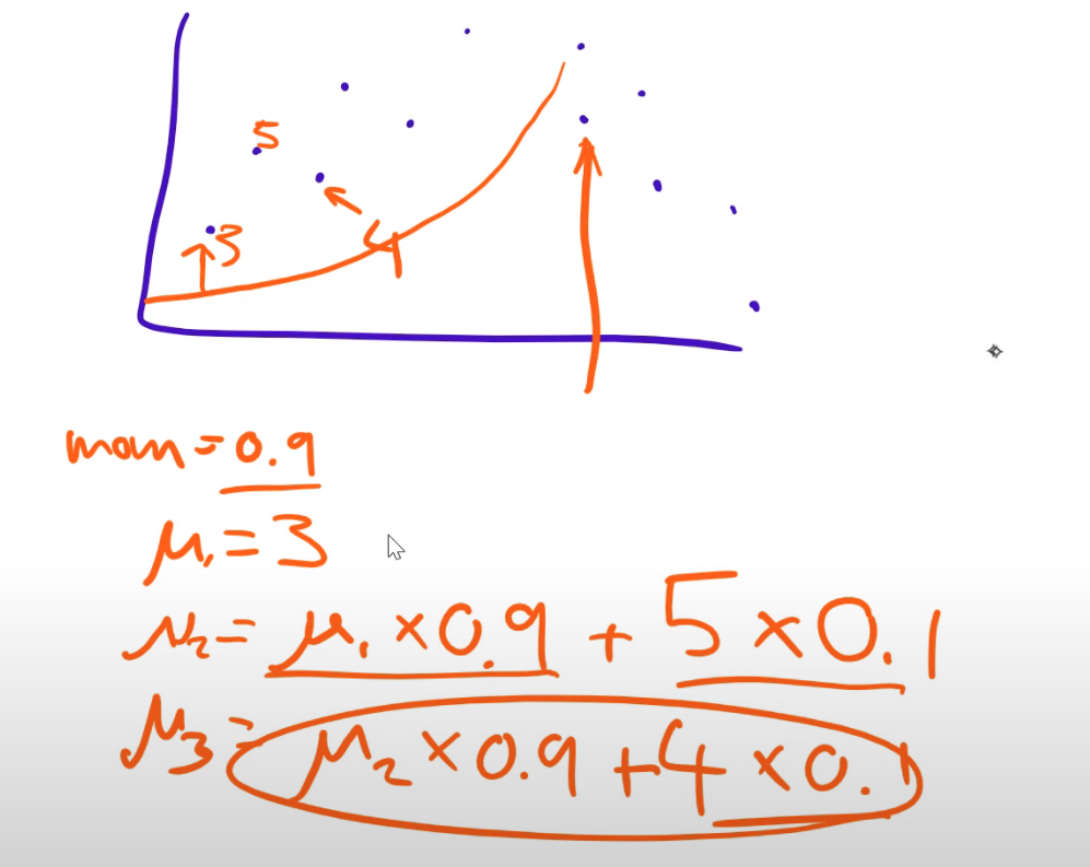
Exponential moving average
We use exp. moving average, that way we only need to keep track of one element.The next value is computed with linear interpolation. PyTorch mom=0.1 is actually 0.9 in math terms. (1-mom)
Now we define our batch norm conv_layer, when we use batch norm we can remove the bias layer as batch norm adds are a bias.
#collapse_show
def conv_layer(ni, nf, ks=3, stride=2, bn=True, **kwargs):
    # No bias needed if using bn
    layers = [nn.Conv2d(ni, nf, ks, padding=ks//2, stride=stride, bias=not bn),
              GeneralRelu(**kwargs)]
    if bn: layers.append(BatchNorm(nf))
    return nn.Sequential(*layers)
#collapse_show
def init_cnn_(m, f):
    if isinstance(m, nn.Conv2d):
        f(m.weight, a=0.1)
        if getattr(m, 'bias', None) is not None: m.bias.data.zero_()
    for l in m.children(): init_cnn_(l, f)

def init_cnn(m, uniform=False):
    f = init.kaiming_uniform_ if uniform else init.kaiming_normal_
    init_cnn_(m, f)

def get_learn_run(nfs, data, lr, layer, cbs=None, opt_func=None, uniform=False, **kwargs):
    model = get_cnn_model(data, nfs, layer, **kwargs)
    init_cnn(model, uniform=uniform)
    return get_runner(model, data, lr=lr, cbs=cbs, opt_func=opt_func)
Above the modules are initalized recursively. We can then use it in training and see how it helps keep the activations means to 0 and the std to 1.
#collapse
learn,run = get_learn_run(nfs, data, 0.9, conv_layer, cbs=cbfs)
Train with Hooks :
#collapse_show
with Hooks(learn.model, append_stats) as hooks:
    run.fit(1, learn)
    fig,(ax0,ax1) = plt.subplots(1,2, figsize=(10,4))
    for h in hooks[:-1]:
        ms,ss = h.stats
        ax0.plot(ms[:10])
        ax1.plot(ss[:10])
        h.remove()
    plt.legend(range(6));

    fig,(ax0,ax1) = plt.subplots(1,2, figsize=(10,4))
    for h in hooks[:-1]:
        ms,ss = h.stats
        ax0.plot(ms)
        ax1.plot(ss)


#collapse
learn,run = get_learn_run(nfs, data, 1.0, conv_layer, cbs=cbfs)
#collapse
%time run.fit(3, learn)
#collapse_show
def conv_layer(ni, nf, ks=3, stride=2, bn=True, **kwargs):
    layers = [nn.Conv2d(ni, nf, ks, padding=ks//2, stride=stride, bias=not bn),
              GeneralRelu(**kwargs)]
    if bn: layers.append(nn.BatchNorm2d(nf, eps=1e-5, momentum=0.1))
    return nn.Sequential(*layers)
#collapse
learn,run = get_learn_run(nfs, data, 1., conv_layer, cbs=cbfs)
#collapse
%time run.fit(3, learn)
Now let's add the usual warm-up/annealing.
#collapse
sched = combine_scheds([0.3, 0.7], [sched_lin(0.6, 2.), sched_lin(2., 0.1)])
#collapse_show
learn,run = get_learn_run(nfs, data, 0.9, conv_layer, cbs=cbfs
                          +[partial(ParamScheduler,'lr', sched)])
#collapse
run.fit(8, learn)
From the paper: "batch normalization cannot be applied to online learning tasks or to extremely large distributed models where the minibatches have to be small". This is the case for large Nets that only allow for small batch sizes. Also RNNs are a problem, as our for loop can not vary the batch size easily.
General equation for a norm layer with learnable affine:
$$y = \frac{x - \mathrm{E}[x]}{ \sqrt{\mathrm{Var}[x] + \epsilon}} * \gamma + \beta$$
The difference with BatchNorm is
- we don't keep a moving average
- we don't average over the batches dimension but over the hidden dimension, so it's independent of the batch size
#collapse_show
class LayerNorm(nn.Module):
    __constants__ = ['eps']
    def __init__(self, eps=1e-5):
        super().__init__()
        self.eps = eps
        self.mult = nn.Parameter(tensor(1.))
        self.add  = nn.Parameter(tensor(0.))

    def forward(self, x):
        m = x.mean((1,2,3), keepdim=True)
        v = x.var ((1,2,3), keepdim=True)
        x = (x-m) / ((v+self.eps).sqrt())
        return x*self.mult + self.add
Keep in mind that compared to BN we use m = x.mean((1,2,3), keepdim=True) instead of m=x.mean((0,2,3), keepdim=True) and we do not use the exp. moving average. The reason is that every image has it's own mean as we do not use batches anymore.
#collapse
def conv_ln(ni, nf, ks=3, stride=2, bn=True, **kwargs):
    layers = [nn.Conv2d(ni, nf, ks, padding=ks//2, stride=stride, bias=True),
              GeneralRelu(**kwargs)]
    if bn: layers.append(LayerNorm())
    return nn.Sequential(*layers)
#collapse_show
learn,run = get_learn_run(nfs, data, 0.8, conv_ln, cbs=cbfs)
#collapse_show
%time run.fit(3, learn)
Thought experiment: can this distinguish foggy days from sunny days (assuming you're using it before the first conv)?
No we can not, layer norm will lead to the same normalization for both pictures. As we can see LN is not as good as BN, but it can be used for RNNS.
From the paper:
The key difference between contrast and batch normalization is that the latter applies the normalization to a whole batch of images instead for single ones:
\begin{equation}\label{eq:bnorm} y_{tijk} = \frac{x_{tijk} - \mu_{i}}{\sqrt{\sigma_i^2 + \epsilon}}, \quad \mu_i = \frac{1}{HWT}\sum_{t=1}^T\sum_{l=1}^W \sum_{m=1}^H x_{tilm}, \quad \sigma_i^2 = \frac{1}{HWT}\sum_{t=1}^T\sum_{l=1}^W \sum_{m=1}^H (x_{tilm} - mu_i)^2. \end{equation}In order to combine the effects of instance-specific normalization and batch normalization, we propose to replace the latter by the instance normalization (also known as contrast normalization) layer:
\begin{equation}\label{eq:inorm} y_{tijk} = \frac{x_{tijk} - \mu_{ti}}{\sqrt{\sigma_{ti}^2 + \epsilon}}, \quad \mu_{ti} = \frac{1}{HW}\sum_{l=1}^W \sum_{m=1}^H x_{tilm}, \quad \sigma_{ti}^2 = \frac{1}{HW}\sum_{l=1}^W \sum_{m=1}^H (x_{tilm} - mu_{ti})^2. \end{equation}#collapse_show
class InstanceNorm(nn.Module):
__constants__ = ['eps']
def __init__(self, nf, eps=1e-0):
super().__init__()
self.eps = eps
self.mults = nn.Parameter(torch.ones (nf,1,1))
self.adds = nn.Parameter(torch.zeros(nf,1,1))
def forward(self, x):
m = x.mean((2,3), keepdim=True)
v = x.var ((2,3), keepdim=True)
res = (x-m) / ((v+self.eps).sqrt())
return res*self.mults + self.adds
Keep in mind that compared to LN we use m = x.mean((2,3), keepdim=True) instead of m=x.mean((1,2,3), keepdim=True).
#collapse
def conv_in(ni, nf, ks=3, stride=2, bn=True, **kwargs):
    layers = [nn.Conv2d(ni, nf, ks, padding=ks//2, stride=stride, bias=True),
              GeneralRelu(**kwargs)]
    if bn: layers.append(InstanceNorm(nf))
    return nn.Sequential(*layers)
#collapse
learn,run = get_learn_run(nfs, data, 0.1, conv_in, cbs=cbfs)
#collapse
%time run.fit(3, learn)
Question: why can't this classify anything?
We are now using the mean and variance for every image and every channel, throwing away the things that allow classification.
It was not designed for Classification, but rather for style transfer where the differences in contrast and overall amount are not important according to the authors.
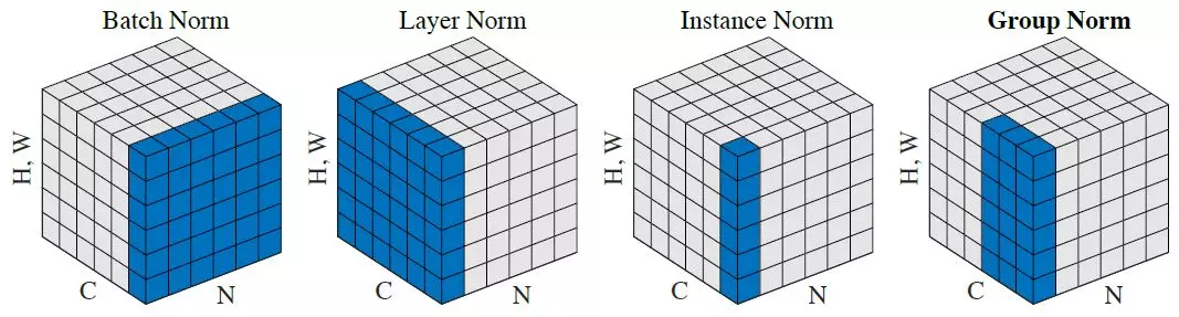
Lost in all those norms? The authors from the group norm paper have you covered:
From the PyTorch docs:
GroupNorm(num_groups, num_channels, eps=1e-5, affine=True)
The input channels are separated into num_groups groups, each containing
num_channels / num_groups channels. The mean and standard-deviation are calculated
separately over the each group. $\gamma$ and $\beta$ are learnable
per-channel affine transform parameter vectorss of size num_channels if
affine is True.
This layer uses statistics computed from input data in both training and evaluation modes.
Args:
- num_groups (int): number of groups to separate the channels into
- num_channels (int): number of channels expected in input
- eps: a value added to the denominator for numerical stability. Default: 1e-5
- affine: a boolean value that when set to
True, this module has learnable per-channel affine parameters initialized to ones (for weights) and zeros (for biases). Default:True.
Shape:
- Input:
(N, num_channels, *) - Output:
(N, num_channels, *)(same shape as input)
Examples::
>>> input = torch.randn(20, 6, 10, 10)
>>> # Separate 6 channels into 3 groups
>>> m = nn.GroupNorm(3, 6)
>>> # Separate 6 channels into 6 groups (equivalent with InstanceNorm)
>>> m = nn.GroupNorm(6, 6)
>>> # Put all 6 channels into a single group (equivalent with LayerNorm)
>>> m = nn.GroupNorm(1, 6)
>>> # Activating the module
>>> output = m(input)When we compute the statistics (mean and std) for a BatchNorm Layer on a small batch, it is possible that we get a standard deviation very close to 0. because there aren't many samples (the variance of one thing is 0. since it's equal to its mean).
#collapse
data = DataBunch(*get_dls(train_ds, valid_ds, 2), c)
#collapse_show
def conv_layer(ni, nf, ks=3, stride=2, bn=True, **kwargs):
    layers = [nn.Conv2d(ni, nf, ks, padding=ks//2, stride=stride, bias=not bn),
              GeneralRelu(**kwargs)]
    if bn: layers.append(nn.BatchNorm2d(nf, eps=1e-5, momentum=0.1))
    return nn.Sequential(*layers)
#collapse
learn,run = get_learn_run(nfs, data, 0.4, conv_layer, cbs=cbfs)
#collapse
%time run.fit(1, learn)
To solve this problem we introduce a Running BatchNorm that uses smoother running mean and variance for the mean and std. Eps is used to avoid divergence, it is used as a hyperparameter. Running Batch Norm is a good solution (best so far according to Jeremy) for the small batch size problem.
1) It does not divide by the batch standard deviation, but it uses the moving average stats at training time as well, just like during inference. Accuracy increases a lot ! As we should not compute the running average of the variances, especially as there might be different batch sizes as well. We use the formula :
$E[X^{2}]-E[X]^{2}$
So we use the squares and the sums with a buffer.
2) And then we take the exp. moving average of these and interpolate. We also take the exponential moving average of the batch sizes, it tells us what we need to divide by : (total number of elements by the mini batch divided by number of channels)
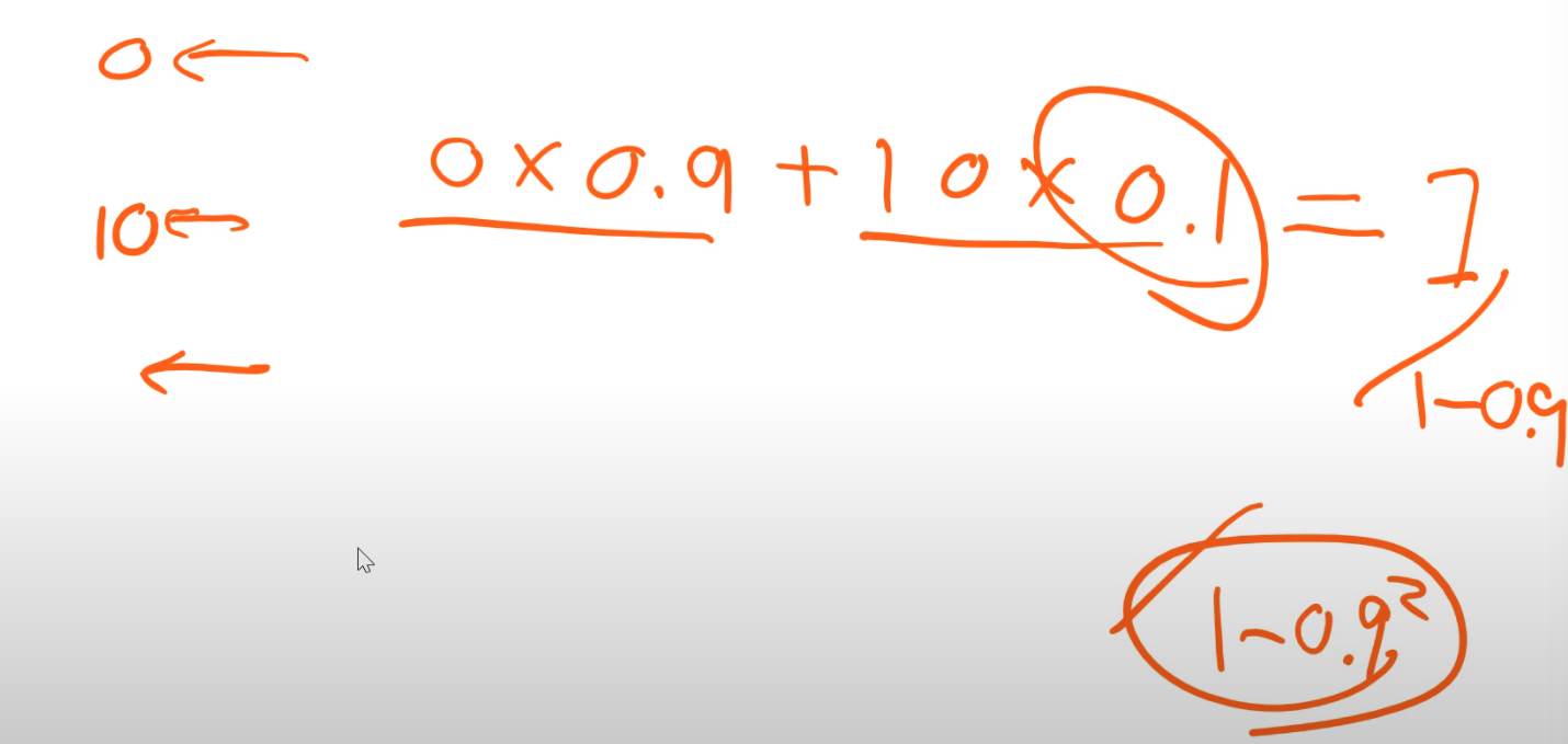
3) Debiasing
Make sure that at every point, no observation is weighted too much. (early elements have more relevance as they appear more often)
4) For the first elements : We might be unlucky, so that our first mini batch is very close to zero. So we clamp the first few elements (for example 20) variance to be 0.01.
#collapse_show
class RunningBatchNorm(nn.Module):
    def __init__(self, nf, mom=0.1, eps=1e-5):
        super().__init__()
        self.mom,self.eps = mom,eps
        self.mults = nn.Parameter(torch.ones (nf,1,1))
        self.adds = nn.Parameter(torch.zeros(nf,1,1))
        self.register_buffer('sums', torch.zeros(1,nf,1,1))
        self.register_buffer('sqrs', torch.zeros(1,nf,1,1))
        self.register_buffer('batch', tensor(0.))
        self.register_buffer('count', tensor(0.))
        self.register_buffer('step', tensor(0.))
        self.register_buffer('dbias', tensor(0.))

    def update_stats(self, x):
        bs,nc,*_ = x.shape
        self.sums.detach_()
        self.sqrs.detach_()
        dims = (0,2,3)
        s = x.sum(dims, keepdim=True)
        ss = (x*x).sum(dims, keepdim=True)
        c = self.count.new_tensor(x.numel()/nc)
        mom1 = 1 - (1-self.mom)/math.sqrt(bs-1)
        self.mom1 = self.dbias.new_tensor(mom1)
        self.sums.lerp_(s, self.mom1)
        self.sqrs.lerp_(ss, self.mom1)
        self.count.lerp_(c, self.mom1)
        self.dbias = self.dbias*(1-self.mom1) + self.mom1
        self.batch += bs
        self.step += 1

    def forward(self, x):
        if self.training: self.update_stats(x)
        sums = self.sums
        sqrs = self.sqrs
        c = self.count
        if self.step<100:
            sums = sums / self.dbias
            sqrs = sqrs / self.dbias
            c    = c    / self.dbias
        means = sums/c
        vars = (sqrs/c).sub_(means*means)
        if bool(self.batch < 20): vars.clamp_min_(0.01)
        x = (x-means).div_((vars.add_(self.eps)).sqrt())
        return x.mul_(self.mults).add_(self.adds)
#collapse_show
def get_cnn_layers(data, nfs, layer,conv_dim,n_res_block, **kwargs):
    nfs = [1] + nfs
    res = resblocks_create(conv_dim,1)
    print(res)
    layers= [layer(nfs[i], nfs[i+1], 5 if i==0 else 3, **kwargs)
            for i in range(len(nfs)-1)] + list(res) + [nn.AdaptiveAvgPool2d(1), Lambda(flatten),nn.Dropout(0.4),
        nn.Linear(nfs[-1], data.c)]
    print(layers)
    return layers

def conv_layer(ni, nf, ks=3, stride=2, **kwargs):
    return nn.Sequential(
        nn.Conv2d(ni, nf, ks, padding=ks//2, stride=stride), GeneralRelu(**kwargs))

class GeneralRelu(nn.Module):
    def __init__(self, leak=None, sub=None, maxv=None):
        super().__init__()
        self.leak,self.sub,self.maxv = leak,sub,maxv

    def forward(self, x):
        x = F.leaky_relu(x,self.leak) if self.leak is not None else F.relu(x)
        if self.sub is not None: x.sub_(self.sub)
        if self.maxv is not None: x.clamp_max_(self.maxv)
        return x

def init_cnn_(m,f):
    if isinstance(m,nn.Conv2d):
            f(m.weight,a = 0.1)
            if getattr(m,'bias',None) is not None : m.bias.data.zero_()
    for l in m.children() : init_cnn_(l,f)

def init_cnn(m, uniform=False):
    f = init.kaiming_uniform_ if uniform else init.kaiming_normal_
    init_cnn_(m,f)

def get_cnn_model(data, nfs, layer,conv_dim,n_res_block, **kwargs):
    return nn.Sequential(*get_cnn_layers(data, nfs, layer,conv_dim,n_res_block, **kwargs))
#collapse_show
class Runner():
    def __init__(self, cbs=None, cb_funcs=None):
        cbs = listify(cbs)
        for cbf in listify(cb_funcs):
            cb = cbf()
            setattr(self, cb.name, cb)
            cbs.append(cb)
        self.stop,self.cbs = False,[TrainEvalCallback()]+cbs

    @property
    def opt(self):       return self.learn.opt
    @property
    def model(self):     return self.learn.model
    @property
    def loss_func(self): return self.learn.loss_func
    @property
    def data(self):      return self.learn.data

    def one_batch(self, xb, yb):
        try:
            self.xb,self.yb = xb,yb
            self('begin_batch')
            self.pred = self.model(self.xb)
            self('after_pred')
            self.loss = self.loss_func(self.pred, self.yb)
            self('after_loss')
            if not self.in_train: return
            self.loss.backward()
            self('after_backward')
            self.opt.step()
            self('after_step')
            self.opt.zero_grad()
        except CancelBatchException: self('after_cancel_batch')
        finally: self('after_batch')

    def all_batches(self, dl):
        self.iters = len(dl)
        try:
            for xb,yb in dl:
                print('Batch')
                self.one_batch(xb, yb)
        except CancelEpochException: self('after_cancel_epoch')

    def fit(self, epochs, learn):
        self.epochs,self.learn,self.loss = epochs,learn,tensor(0.)

        try:
            for cb in self.cbs: cb.set_runner(self)
            self('begin_fit')
            for epoch in range(epochs):
                self.epoch = epoch
                if not self('begin_epoch'): self.all_batches(self.data.train_dl)

                with torch.no_grad():
                    if not self('begin_validate'): self.all_batches(self.data.valid_dl)
                self('after_epoch')

        except CancelTrainException: self('after_cancel_train')
        finally:
            self('after_fit')
            self.learn = None

    def __call__(self, cb_name):
        res = False
        for cb in sorted(self.cbs, key=lambda x: x._order): res = cb(cb_name) or res
        return res
If you recall from the lecture, a simple CNN is used. The goal was to improve one epoch training validation error as a practice toy problem. I did beat the 0.975 slightly from the video with Dropout in the fully connected part, but further added a Residual block after the normal Conv Part, allowing u.
#collapse_show
def get_runner(model, data, lr=0.6, cbs=None, opt_func=None, loss_func = F.cross_entropy):
    if opt_func is None: opt_func = optim.SGD
    opt = opt_func(model.parameters(), lr=lr)
    learn = Learner(model, opt, loss_func, data)
    return learn, Runner(cb_funcs=listify(cbs))
#collapse_show
def conv(in_channels, out_channels, kernel_size, stride=2, padding=1, batch_norm=True):
    """Creates a convolutional layer, with optional batch normalization.
    """
    layers = []
    conv_layer = nn.Conv2d(in_channels=in_channels, out_channels=out_channels,
                           kernel_size=kernel_size, stride=stride, padding=padding, bias=False)

    layers.append(conv_layer)

    if batch_norm:
        layers.append(nn.BatchNorm2d(out_channels))
    return nn.Sequential(*layers)
#collapse_show
class Resblock(nn.Module):
    def __init__(self,conv_dim):
        super(Resblock,self).__init__()
        self.conv1 = conv(conv_dim, conv_dim, kernel_size=3, stride=2, batch_norm=True)
        self.conv2 = conv(conv_dim, conv_dim, kernel_size=3, stride=2, batch_norm=True)
    def forward(self,x):
        out1 = F.leaky_relu(self.conv1(x))
        out =  x + F.leaky_relu(self.conv2(out1))
        return out
#collapse_show
def resblocks_create(conv_dim,n_res_blocks):
    res_layers = []
    for l in range(0,n_res_blocks):
        res_layers.append(Resblock(conv_dim))
    return nn.Sequential(*res_layers)
#collapse_show
def conv_rbn(ni, nf, ks=3, stride=2, bn=True, **kwargs):
    layers = [nn.Conv2d(ni, nf, ks, padding=ks//2, stride=stride, bias=not bn),
              GeneralRelu(**kwargs)]
    if bn: layers.append(RunningBatchNorm(nf))
    print(**kwargs)
    return nn.Sequential(*layers)
#collapse
def get_learn_run(nfs, data,conv_dim,n_res_block, lr, layer, cbs=None, opt_func=None, uniform=False, **kwargs):
    model = get_cnn_model(data, nfs, layer,conv_dim,n_res_block, **kwargs)
    init_cnn(model, uniform=False)
    return get_runner(model, data, lr=lr, cbs=cbs, opt_func=opt_func)
#collapse
nfs = [8,16,32,64]
#collapse
learn,run = get_learn_run(nfs, data, 64,1,0.4, conv_rbn, cbs=cbfs)
learn.model
#collapse
%time run.fit(1, learn)
This solves the small batch size issue!
Now let's see with a decent batch size what result we can get.
#collapse
data = DataBunch(*get_dls(train_ds, valid_ds, 16), c)
#collapse
learn,run = get_learn_run(nfs, data, 64,1, 0.9, conv_rbn, cbs=cbfs
                          +[partial(ParamScheduler,'lr', sched_lin(1., 0.2))])
#collapse
%time run.fit(1, learn)